chess recognition
If you’re a recreational chess player, the following scenario will likely sound familiar: you’re plaing a casual over-the-board game, and reach an interesting position. You may even be thinking about a spicy piece sacrifice. Long story short, you want to perform a computer analysis after the game, to see if you made the right decision. So, you take a picture of the current position before proceeding with the game.
After the game, you can use this picture to enter the position into a chess analysis program, like the popular analysis board tool on Lichess. However, this process is time-consuming and error-prone – you need to drag & drop pieces around the board, until reaching the position you had in the photo.
With all the recent (and not-so-recent) advances in deep learning and computer vision, you’d think it would be possible to automate this tedious procedure. Enter chesscog, an end-to-end chess recognition system I developed as part of my master’s thesis at the University of St Andrews and published as a journal article [1]. The goal of this project was to develop a system that is able to map a photo of a chess position to a structured format that can be understood by chess engines, such as the widely-used Forsyth-Edwards Notation (FEN). Perhaps the problem is best explained by a screenshot of the solution (a demo app) below.
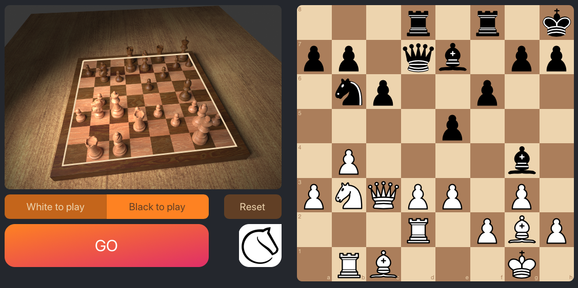
How does it work? I’ll give you the short version in this blog post; if you’re interested, check out my master’s thesis, the associated paper, and the code on GitHub.
Method
When you think about the problem, it seems logical to decompose it into three steps:
-
Board localisation. First, we need to localise the board, i.e. determine the four corner points. This is done using traditional computer vision techniques such as Canny edge detection [2], Hough transform [3], and RANSAC [4].
Once the corner points are established, we can perform some simple geometric calculations to compute the nine horizontal and vertical grid lines, taking into account perspective distortion (the camera parameters are not required for this). It actually turns out that it is more convenient to remove the perspective distortion by projecting the localised chessboard onto a regular square grid.
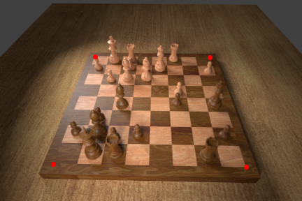
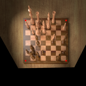 The perspective distortion is removed from the left image by projecting the four corner points onto a square grid (right).
 -
Occupancy classification. Next, we can crop out each of the chess squares from the un-distorted image, and feed them into a convolutional neural network (CNN) acting as a binary classifier between empty and occupied squares. It turns out that performing this step prior to the piece classification significantly increases accuracy (as opposed to considering the empty square as a piece type).
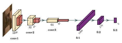 Example of an occupancy classification CNN that distinguishes between empty and occupied squares.
 -
Piece classification. Finally, the occupied samples are fed through another (larger) CNN that performs a 12-way classification to determine piece colour (black or white), and piece type (pawn, knight, bishop, rook, queen, or king). The predictions are gathered for each of the 64 squares and used to generate the corresponding FEN string.
Training
In order to train the CNNs, a dataset is required. The lack of sizable and adequately labelled datasets is an issue recognised by several prior works [5], [6], [7]. Instead of manually creating a dataset and labelling it, I modelled a chess set in Blender, and created a Python script render ~5,000 synthetic chessboard images with different camera poses, lighting conditions, and game states. This approach allowed me to create a much larger dataset for chess recognition – I made it publicly available here [8], to aid future research and enable fair comparison over a common dataset.
I trained the occupancy classification and piece classification CNNs separately on the synthesised dataset. I tried out various hyperparameters and initialisations, and achieved the best results with models that were pre-traind on ImageNet. In the end, the system achieved an error rate of 0.23% per square on the test set, 28 times better than the previous state of the art [7].
Adapting to unseen chess sets
The last piece of the puzzle comes with the realisation that every chess set has a different appearance – different shapes, materials, colours, etc. The pipeline described above does not work very well out-of-the-box on unseen real-life chess sets because it was only trained on synthetic images. So, how do we adapt to an unseen chess set?
At this point it is important to note that the first step in the pipeline does actually work quite well on unseen chess sets, due to the use of traditional computer vision techniques (as opposed to learned features). This means that we can actually perform the perspective unwarping, and extract the 64 squares from practically any input image of a chess set.
This lead me to the idea to ask the user to supply two pictures to fine-tune the CNNs to any new chess set. These two pictures should be of the starting position, once each players perspective. Using the board localisation algorithm, it turns out that just these two images can generate enough training data to fine-tune the two CNNs (keep in mind that each image generates 64 samples of chess squares), although careful data augmentations were required to achieve good results. The CNNs were initialised with the trained weights from the synthesised dataset, and then fine-tuned using the newly cropped and augmented images.
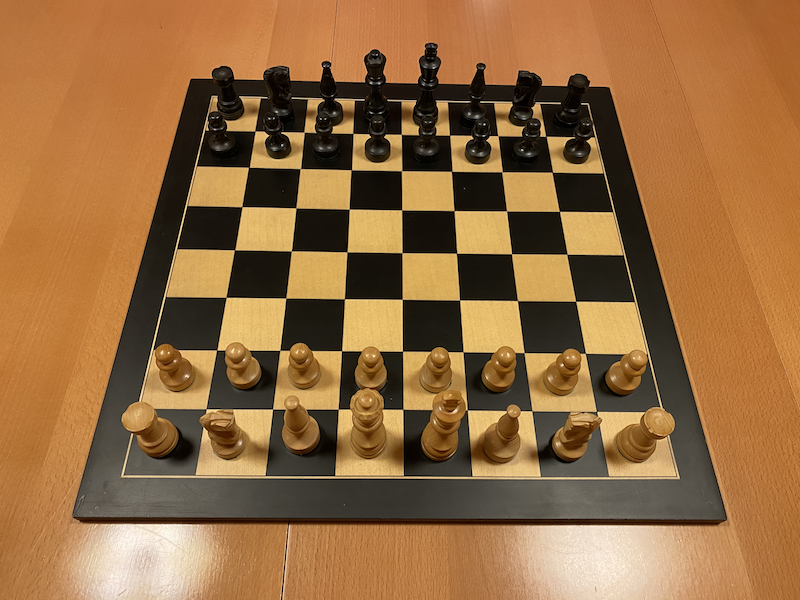
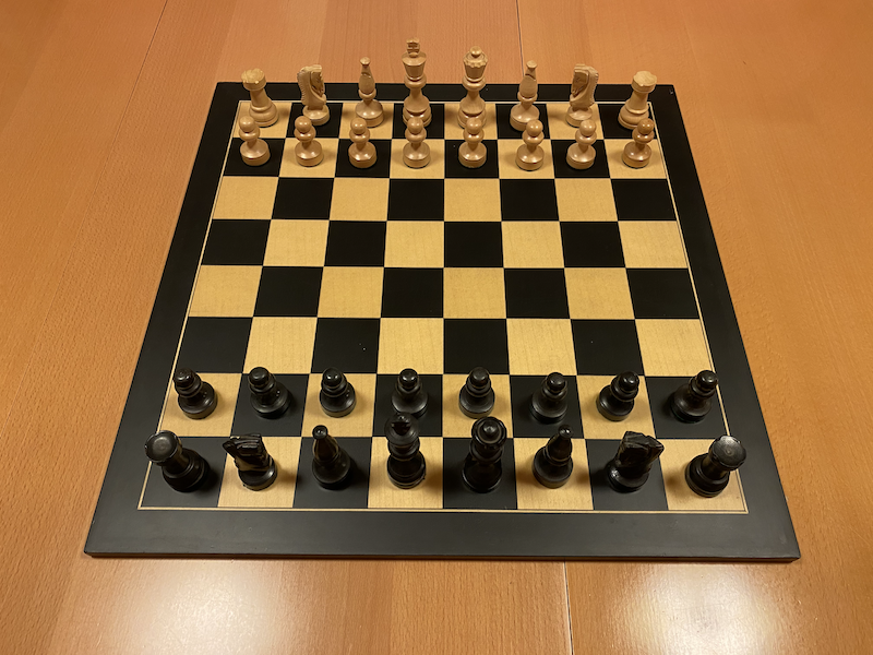
In the evaluation, the fine-tuning dataset consisted of the two images depicted above, and the test dataset contained 27 images obtained by playing a game of chess and taking a picture after each move. Even on this unseen dataset, the chess recognition pipeline achieved very convincing results. The per-square misclassification rate was just 0.17% on the test set. See the table below for a summary of the results.

What’s next?
There are plenty avenues to continue this research, below I’ll name a few:
- Improve the process of adapting to unseen chess sets, for example by employing meta-learning to reduce the number of steps needed to fine-tune the network.
- Train on a more diverse dataset of real-world images, to eliminate the need for fine-tuning entirely.
- Devise a differentiable pipeline that can be trained end-to-end (as opposed to the three steps outlined in this blog post which are trained separately).
- Improve the web app (it currently runs in Heroku’s free tier on a single CPU, frequently running into out-of-memory errors).
If you’re keen on helping on any of these points, or have other suggestions, drop me an email!
Further links
- The chesscog app.
- The code is available on GitHub.
- My article in the Journal of Imaging, “Determining Chess Game State From an Image”.
- My master’s thesis, which goes into more detail than this blog post and the journal article.
References
- G. Wölflein and O. Arandjelović, “Determining Chess Game State from an Image,” Journal of Imaging, vol. 7, no. 6, 2021.
- J. Canny, “A Computational Approach to Edge Detection,” IEEE Transactions on Pattern Analysis and Machine Intelligence, 1986.
- R. O. Duda and P. E. Hart, “Use of the Hough Transformation to Detect Lines and Curves in Pictures,” Communications of the ACM, vol. 15, no. 1, 1972.
- M. A. Fischler and R. C. Bolles, “Random Sample Consensus: A Paradigm for Model Fitting with Applications to Image Analysis and Automated Cartography,” Communications of the ACM, vol. 24, no. 6, 1981.
- J. Ding, “ChessVision: Chess Board and Piece Recognition.” Stanford University, 2016.
- M. A. Czyzewski, A. Laskowski, and S. Wasik, “Chessboard and Chess Piece Recognition with the Support of Neural Networks.” 2020.
- A. Mehta and H. Mehta, “Augmented Reality Chess Analyzer (ARChessAnalyzer),” Journal of Emerging Investigators, vol. 2, 2020.
- G. Wölflein and O. Arandjelović, “Dataset of Rendered Chess Game State Images.” Open Science Framework, 2021. doi: 10.17605/OSF.IO/XF3KA.